Simple examples of perturbation theory

3.1.1 Simple examples of perturbation theory

Probably the simplest example we can think of is an inﬁnite square well with a low step half way across, so that $V (x) = 0$ for $0 < x < a ∕ 2$ , $V_{0}$ for $a ∕ 2 < x < a$ and inﬁnite elsewhere. We treat this as a perturbation on the ﬂat-bottomed well, so $H^{(1)} = V_{0}$ for $a ∕ 2 < x < a$ and zero elsewhere.

The ground-state unperturbed wavefunction is $ψ_{0}^{(0)} = \sqrt{\frac{2}{a}} sin \frac{π x}{a}$ , with unperturbed energy $E_{0}^{(0)} = π^{2} ℏ^{2} ∕ (2 m a^{2})$ . A “low” step will mean $V_{0} ≪ E_{0}^{(0)}$ . Then we have

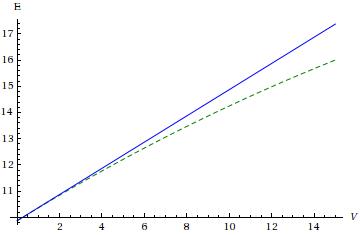
E_{0}^{(1)} = ⟨ ψ_{0}^{(0)} | H^{(1)} | ψ_{0}^{(0)} ⟩ = \frac{2}{a} \int_{a ∕ 2}^{a} V_{0} {sin}^{2} \frac{π x}{a} d x = \frac{V_{0}}{2}

This problem can be solved semi-analytically; in both regions the solutions are sinusoids, but with wavenumbers $k = \sqrt{2 m E} ∕ ℏ$ and $k^{'} = \sqrt{2 m (E - V_{0})} ∕ ℏ$ respectively; satisfying the boundary conditions and matching the wavefunctions and derivatives at $x = a ∕ 2$ gives the condition $k cot (k a ∕ 2) = k^{'} cot (k^{'} a ∕ 2)$ which can be solved numerically for $E$ . (You ought to try this, it will be good practice for later sections of the course.) Below the exact solution (green, dotted) and $E_{0}^{(0)} + E_{0}^{(1)}$ (blue) are plotted; we can see that they start to diverge when $V_{0} = 5$ (everything is in units of $ℏ^{2} ∕ (2 m a^{2})$ ).

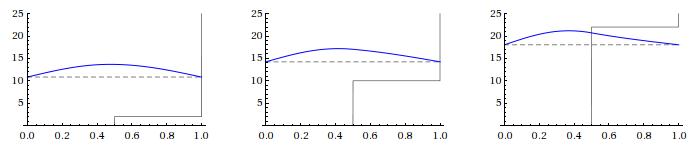
We can also plot the exact wavefunctions for diﬀerent step size, and see that for $V_{0} = 10$ (the middle picture, well beyond the validity of ﬁrst-order perturbation theory) it is signiﬁcantly diﬀerent from a simple sinusoid.

Another example is the harmonic oscillator, with a perturbing potential $H^{(1)} = λ x^{2}$ . The states of the unperturbed oscillator are denoted $| n^{(0)} ⟩$ with energies $E_{0}^{(0)} = (n + \frac{1}{2}) ℏ ω$ .

Recalling that in terms of creation and annihilation operators (see section A.4), $\hat{x} = \sqrt{ℏ ∕ (2 m ω)} (â + â^{†})$ , with $[â, â^{†}] = 1$ , and so

E_{n}^{(1)} = ⟨ n^{(0)} | H^{(1)} | n^{(0)} ⟩ = \frac{ℏ λ}{2 m ω} ⟨ n^{(0)} | {(â^{†})}^{2} + â^{2} + 2 â^{†} â + 1 | n^{(0)} ⟩ = \frac{λ}{m ω^{2}} ℏ ω (n + \frac{1}{2})

The ﬁrst-order change in the wavefunction is also easy to compute, as $⟨ m^{(0)} | H^{(1)} | n^{(0)} ⟩ = 0$ unless $m = n \pm 2$ . Thus

\begin{array}{rcl} | n^{(1)} ⟩ & = & \sum_{m \neq n} \frac{⟨ m^{(0)} | {\hat{H}}^{(1)} | n^{(0)} ⟩}{E_{n}^{(0)} - E_{m}^{(0)}} | m^{(0)} ⟩ \\ = & \frac{ℏ λ}{2 m ω} (\frac{\sqrt{(n + 1) (n + 2)}}{- 2 ℏ ω} | {(n + 2)}^{(0)} ⟩ + \frac{\sqrt{n (n - 1)}}{2 ℏ ω} | {(n - 2)}^{(0)} ⟩) \\ and E_{n}^{(2)} & = & ⟨ n^{(0)} | {\hat{H}}^{(1)} | n^{(1)} ⟩ = \sum_{m \neq n} \frac{{|⟨ m^{(0)} | {\hat{H}}^{(1)} | n^{(0)} ⟩|}^{2}}{E_{n}^{(0)} - E_{m}^{(0)}} \\ = & {(\frac{ℏ λ}{2 m ω})}^{2} (\frac{(n + 1) (n + 2)}{- 2 ℏ ω} + \frac{n (n - 1)}{2 ℏ ω}) = - \frac{1}{2} {(\frac{λ}{m ω^{2}})}^{2} ℏ ω (n + \frac{1}{2}) \end{array}

We can see a pattern emerging, and of course this is actually a soluble problem, as all that the perturbation has done is change the frequency. Deﬁning $ω^{'} = ω \sqrt{1 + 2 λ ∕ (m ω^{2})}$ , we see that the exact solution is

E_{n} = (n + \frac{1}{2}) ℏ ω^{'} = (n + \frac{1}{2}) ℏ ω (1 + \frac{λ}{m ω^{2}} - \frac{1}{2} {(\frac{λ}{m ω^{2}})}^{2} + \dots)

in agreement with the perturbative calculation.

[up] [top]