Gaussian integrals

A.9 Gaussian integrals

The following integrals will be useful:

\int_{- \infty}^{\infty} e^{- α x^{2}} d x = \sqrt{\frac{π}{α}} and \int_{- \infty}^{\infty} x^{2 n} e^{- α x^{2}} d x = {(- 1)}^{n} \frac{d^{n}}{d α^{n}} (\sqrt{\frac{π}{α}})

Often we are faced with a somewhat more complicated integral, which can be cast in Gaussian form by “completing the square” in the exponent and then shifting integration variable $x \to x - β ∕ (2 α)$ :

\int_{- \infty}^{\infty} e^{- α x^{2} - β x} d x = e^{β^{2} ∕ (4 α)} \int_{- \infty}^{\infty} e^{- α {(x + β ∕ (2 α))}^{2}} d x = \sqrt{\frac{π}{α}} e^{β^{2} ∕ (4 α)}

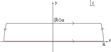
This works even if $β$ is imaginary. One way of seeing this is as follows. In the diagram below, as $R \to \infty$ the blue contour is the original one (with $β$ imaginary) and the red one the new contour after shifting; the red and black paths together must equal the blue since there are no poles in the region bounded by the complete contour. However as $e^{- z^{2}}$ tends to zero faster than $1 ∕ R$ as $R \to \infty$ providing $|x| > |y|$ , the contribution from the black paths is zero. Hence the two integrals must be the same.

[next] [prev] [up] [top]