Real integrals via contour integration
- The contours above are examples of contours which can be used to calculate real integrals
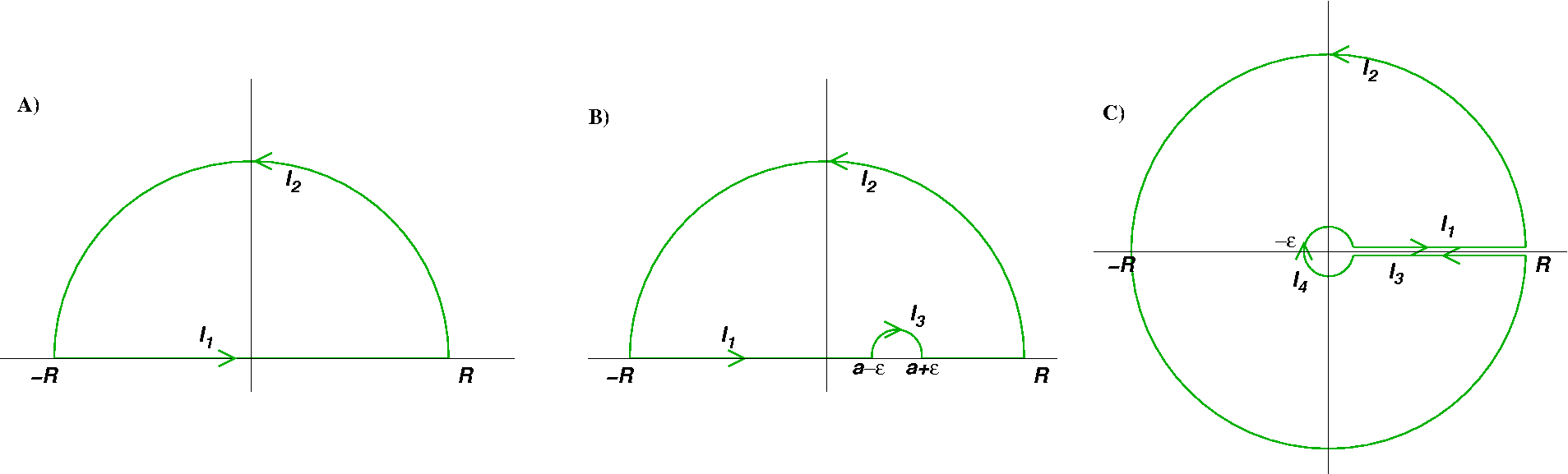
- If $I=\int_{-\infty}^\infty f(x)\d x$, and $f(z)$ has a finite number of poles none of which are on the real axis,
and $|f(R\e^{i\theta})|\to 0$
faster than $1/R$ as $R\to \infty$, then we can use contour $C$ shown in (A). With $R$ large enough
so that all poles in the upper half plane are within $C$, $\lim_{R\to\infty}I_2=0$. Hence
$$ I=\lim_{R\to\infty}I_1= \lim_{R\to\infty}\left(\oint_C f(z)\d z-I_2\right) =2\pi i\text{(Sum of residues at all poles inside $C$)}$$
- If $I=\int_{-\infty}^\infty f(x)\e^{ikx}\d x$, and (i) $k>0$, (ii) $f(z)$ has a finite number of poles in
the upper half plane and (iii) $|f(R\e^{i\theta})|\to 0$ as $R\to \infty$, then we can also
use contour $C$ shown in (A). The vanishing of $I_2$ as $R\to \infty$ in this case is called Jordan's lemma.
If $k<0$, but the other conditions of Jordan's lemma hold for the lower half plane, we can close the contour
in the lower half plane instead.
- If in either case above there is a pole on the real axis at $z=a$, we define the principal value of the integral
to be $\lim_{\epsilon\to 0}\int_{-\infty}^{a-\epsilon} f(x)\d x+\int_{a+\epsilon}^{\infty} f(x)\d x$. To evaluate
it we use the contour shown in (B). If the pole is simple or of odd order we have $\lim_{\epsilon\to 0}I_3=-i\pi\,b_1$
where $b_1$ is the residue of the pole at $z=a$.
If the pole is of even order the principal value of the integral will not exist.
- If the integrand has a branch point at $z=0$ we may be able to evaluate $I=\int_{0}^\infty f(x)\d x$ through
the use of the contour shown in (C), where the branch cut is taken along the positive real axis.
The contributions $I_1$ and $I_3$ will not cancel because $f(x)\ne f(x\e^{2\pi i})$.
- If $I=\int_{0}^{2\pi} F(\sin\theta,\cos\theta)\d \theta$, the integral may be able to be evaluated through
the variable change $z=\e^{i\theta}$ which maps the real $\theta$ integral onto a contour integral round the
unit circle.
- Integrands of the form $f(z) \tan z$, $f(z)/ \sin z$ etc may be used to evaluate series of the
form $\sum_i \pm f(x_i)$ where $x_i$ are the zeros of $\sin x$ or $\cos x$. The relevant contour
integral is
a large circle whose radius $R$ is such that the circle crosses the real axis half way between a pair
of poles. Then provided $f(z)$ falls off faster than $1/R$ as $R\to\infty$, the contour integral will tend to zero.
Spiegel 7.4-8
Riley 18.16-19; Boas 14.7; Arfken 7.2